Coronavirus Pandemic Prediction

Predicting and understanding the spread of the COVID-19 Pandemic in the USA can help forecast supply chains and save jobs and lives.

Predictions made

The past reproduction number is first calculated using estimates based on the SIRf pandemic model. Geographic, Socioeconomic and Health factors from individual counties are sourced and analysed from USA government datasets. These factors are used in machine learning models to predict the spread of the virus. The final results are visualised geographically:

Data Visualisation

Visualising numbers is extremely important when tackling data science problems. Here, folium was used to produce an interactive map to aid our analysis:

Calculating the reproduction number (R)

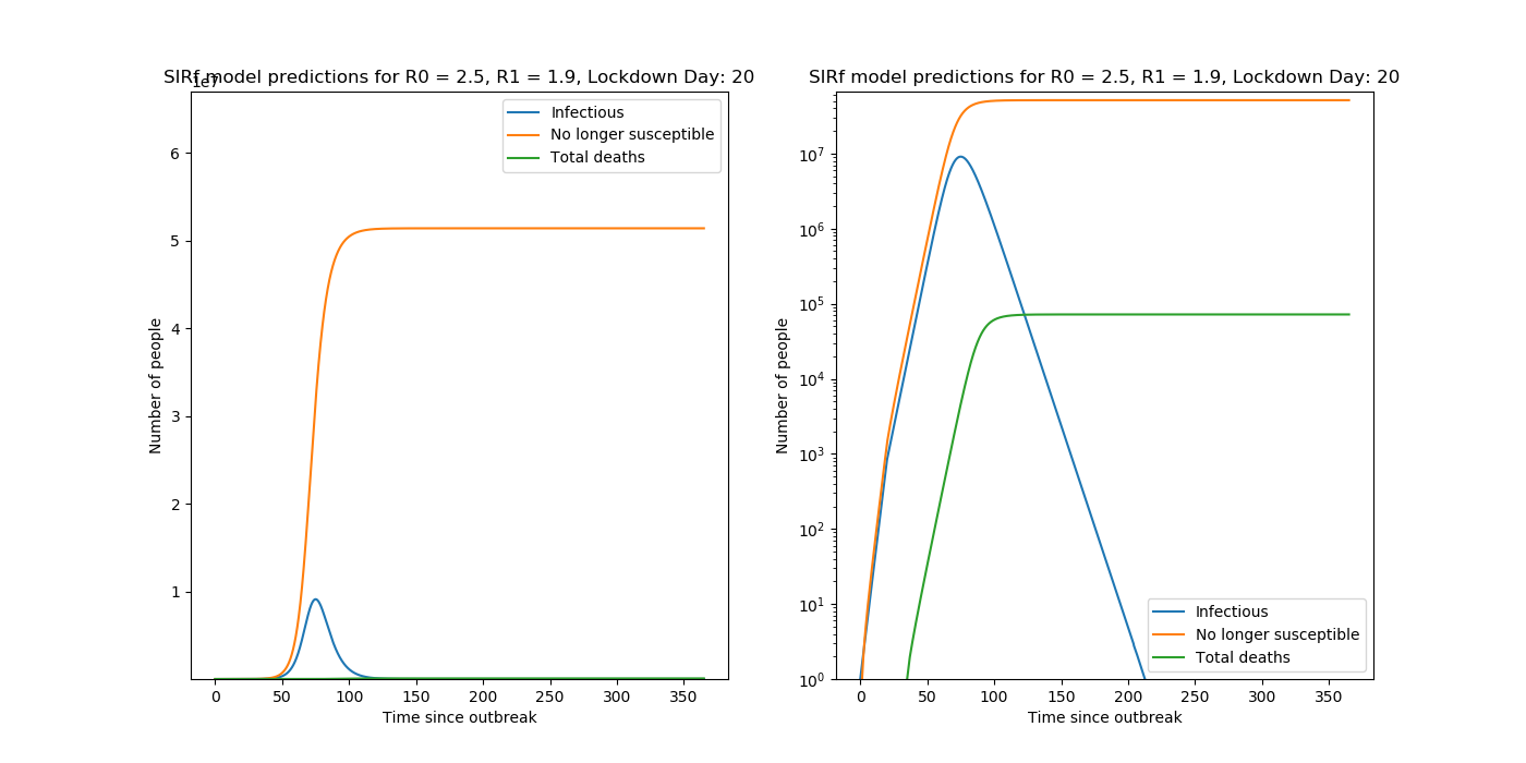
Predictions are made with the following set of coupled ODEs,

\[\frac{dy}{dz} = by(1-z) - \frac{y}{T}\] \[\frac{dz}{dt} = by(1-z)\] \[D = NPaz(t-1)\]

where \(b = \frac{R}{T}\) .

See my post on SIRf Modelling for more details on this model. Other trialled estimates of R included taking ratios of daily case data.

Data Collection

Geographic, Socioeconomic, Ethnic and Health statistics for each indivual county were collected from public datasets listed here. This is a large, unorganised dataset with many missing values and 534 columns! Let’s visualise our data with a sparsity matrix to get an overview and locate missing values:

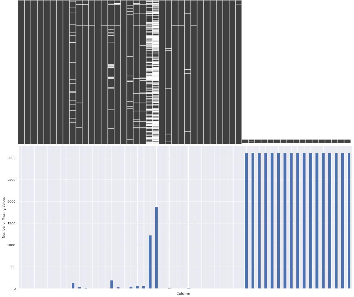
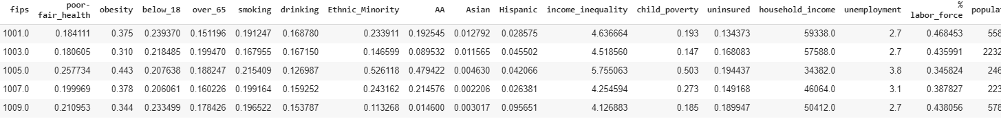
We can see missing values are scattered throughout, but we can now use Pandas to selectively remove and replace values. With some final cleaning, we can extract data for just the factors that we suspect may be interest for further analysis. Factors initially chosen included Obesity, Unemployment, Rurality, Population Density, etc. Here is an example some of the final cleaned data:

Feature Selection

Now we have clean data, but which of these features actually contribute to the spread of Coronavirus? We can use a correlation matrix to quickly identify patterns within:

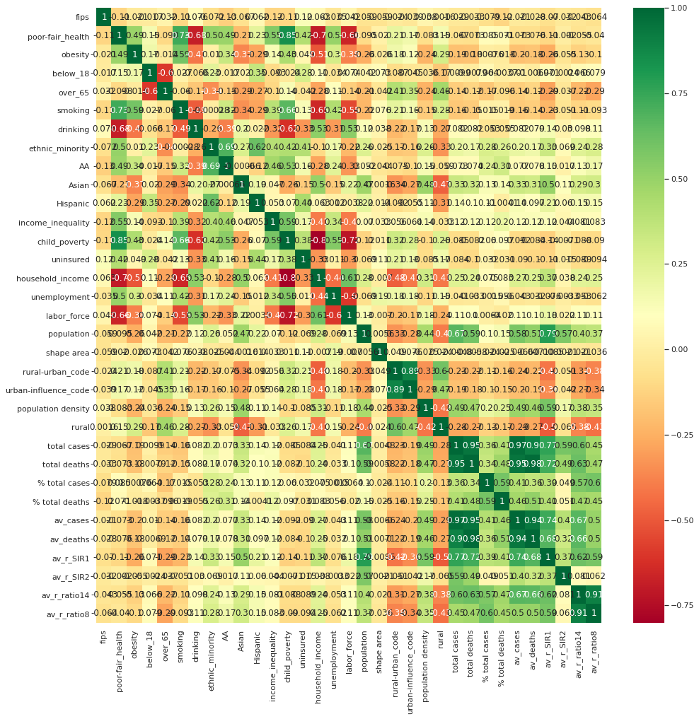
This looks overwhelming, but we can now pick out relationships in our data to explore further:

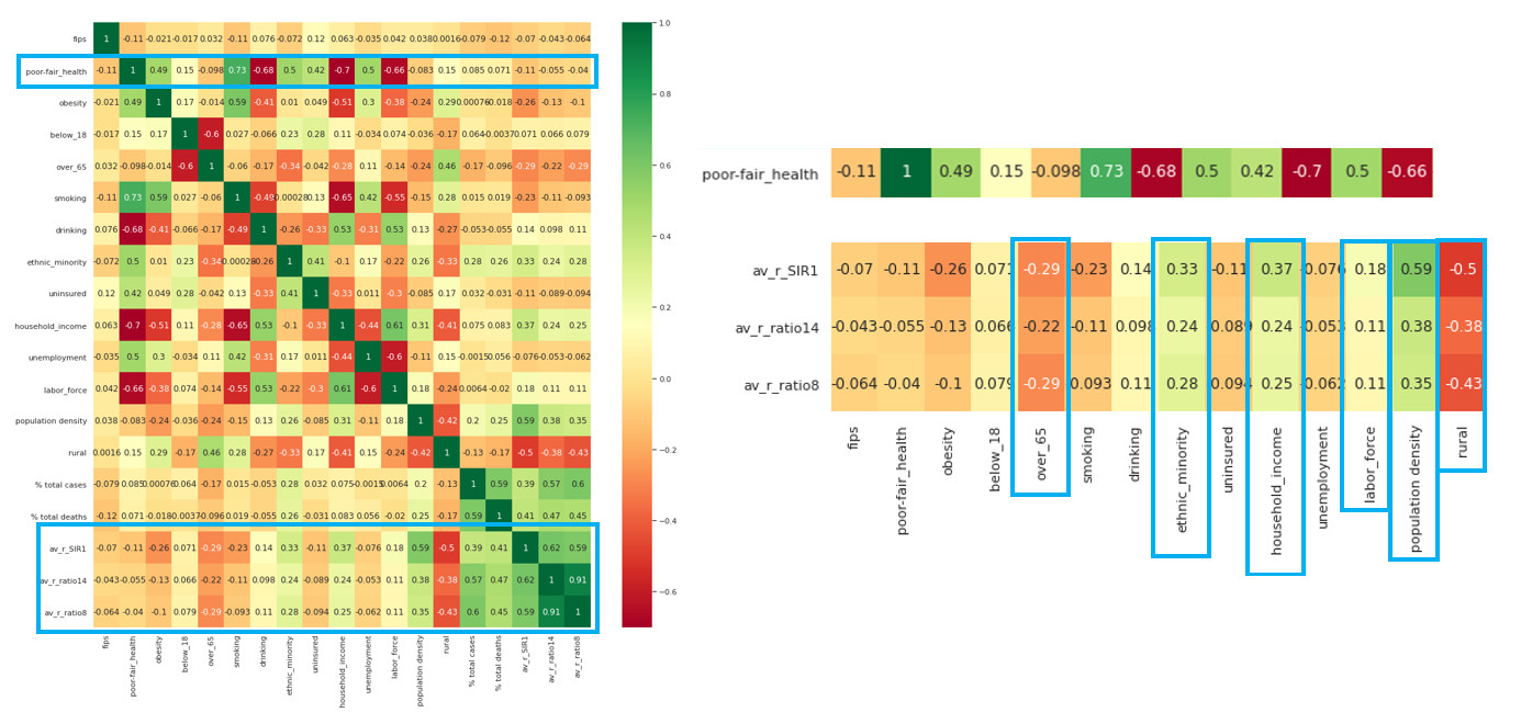
We can plot these factors against the average R rate since the start of the outbreak:

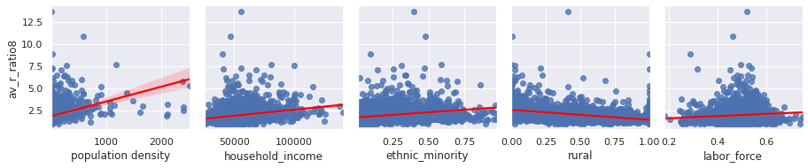
Factors effecting our R rate seem to include population density, rurality, labour face, and interestingly ethnicity. Let’s explore that last factor further:

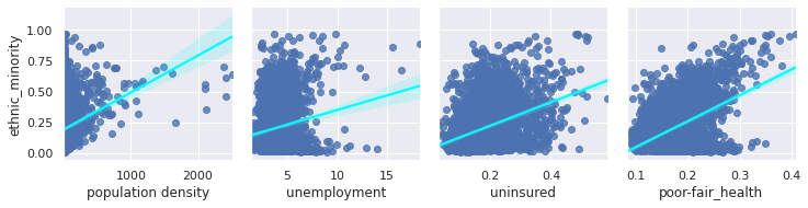
We now see that ethnic minorities tend to live in areas which are more densely populated, likely leading to the false correlation here.

Since population density seems to be important, let’s compare this with the average R rate in each location since the start of the outbreak:

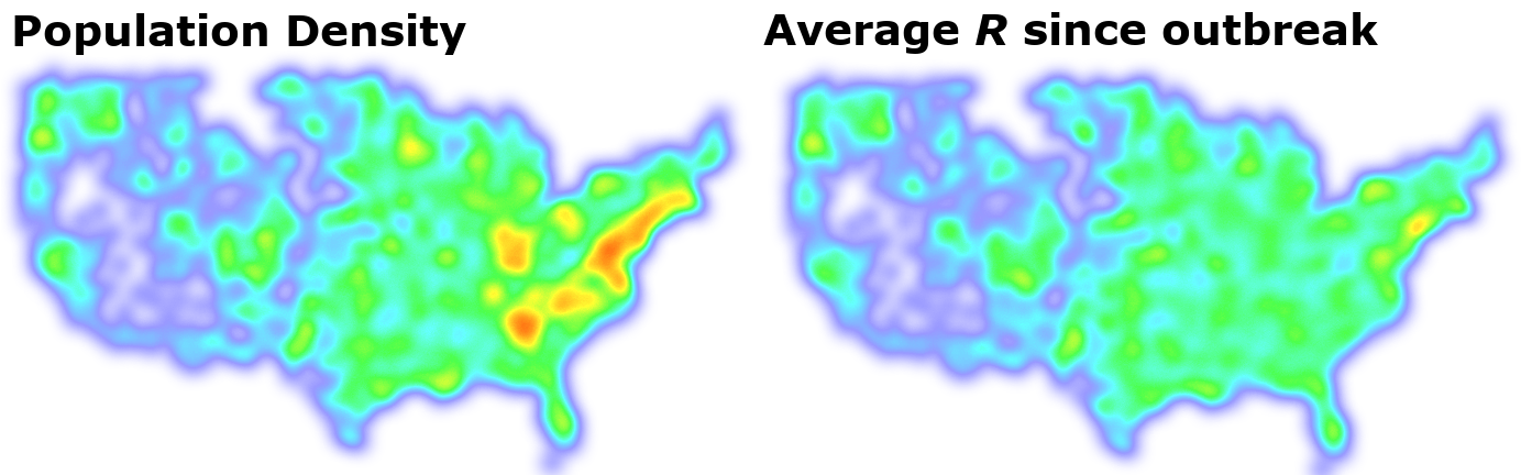
This shows a very strong relationship indeed! These methods allow us to explore interesting relationships and select which factors are important and should be used in our machine learning models to make future predictions.

Machine Learning Predictions

We can now use the information we have on the counties to predict how the virus will spread. We make use of the historical case data along with the extra factors we identified, and hope train a machine learning (ML) model to predict what might happen in the future.

Various machine learning models were explored, and deep learning proved to be very effective. In this approach, we make use on an artificial neural network capable of spotting complex trends in the training data to make predictions. Three network structures were trialled, with increasing complexity :

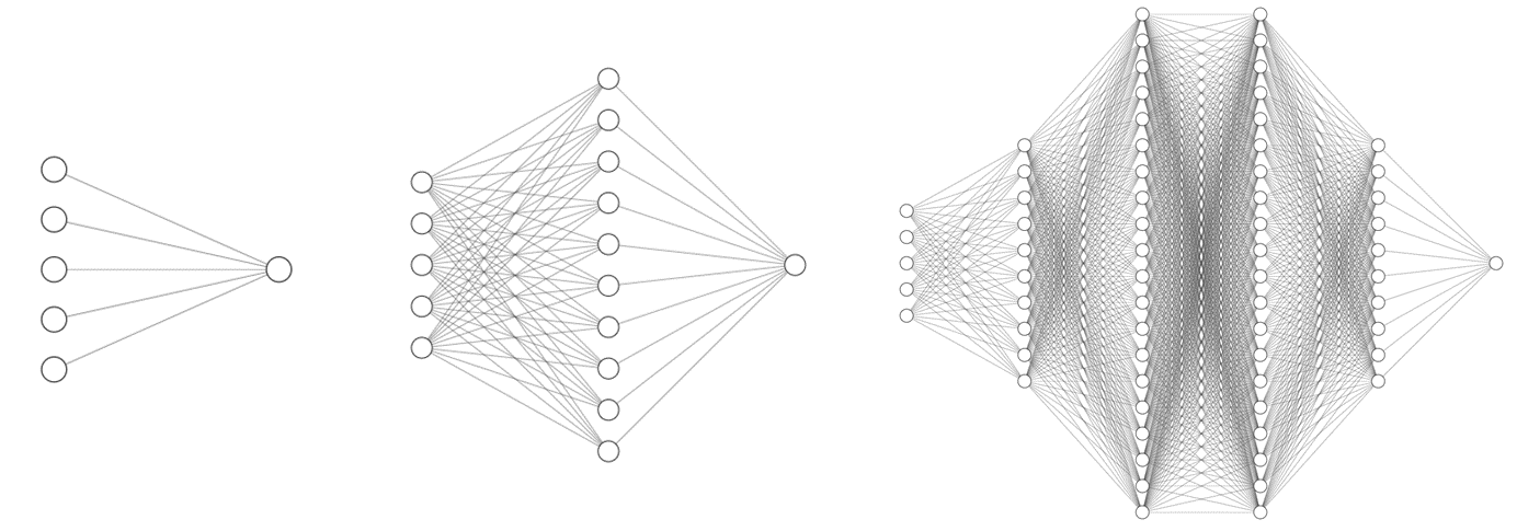
Using keras with a tensorflow backend, we can quickly implement a recurrent neural network:

# Modules
from keras.models import Sequential
from keras.layers import *

# Use a Deep RNN
model = Sequential()

# Input and hidden layers :
model.add(Dense(50, input_dim=num_input_nodes, activation='relu'))
model.add(Dense(100, activation='relu'))
model.add(Dense(100, activation='relu'))
model.add(Dense(50, activation='relu'))

# Output neuron with linear activation function
model.add(Dense(1, activation='linear')) 

# Use MAE for our loss function
model.compile(loss='mean_absolute_error', optimizer='adam')

We pass our training data through the networks, and measure the loss (a measure of how ‘badly’ our model is doing) - which we hope to see decreasing over time as the network learns:

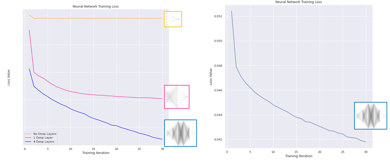
We see the loss decreasing each training iteration; our neural networks are learning trends in our data! Training showed our most complex network performed best, so we will use this for our predictions. We can now use the information we have on the counties to forecast how COVID-19 may spread in the future with our trained model:

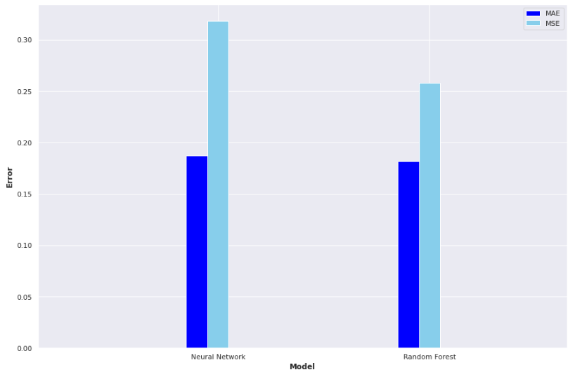
Result! The daily Mean Absolute Error (MAE) of the test set was under 0.2 (each day we are only 0.2 off the true R value in each county, on average). A random forest model, carefully optimised with cross-validation also proved very effective:

This project has displayed that predicting the evolution of a pandemic with ML is feasible and can be used to assist in mitigating the impact of a virus such as COVID-19. I hope this post was interesting and outlined some of the steps involved in a machine learning project. Full source code and further details can be found on my GitHub.